Basic data exploration
Nhi Hin
2021-12-06
Last updated: 2021-12-06
Checks: 7 0
Knit directory: Tom_Proteomics/
This reproducible R Markdown analysis was created with workflowr (version 1.6.2). The Checks tab describes the reproducibility checks that were applied when the results were created. The Past versions tab lists the development history.
Great! Since the R Markdown file has been committed to the Git repository, you know the exact version of the code that produced these results.
Great job! The global environment was empty. Objects defined in the global environment can affect the analysis in your R Markdown file in unknown ways. For reproduciblity it’s best to always run the code in an empty environment.
The command set.seed(20210429) was run prior to running the code in the R Markdown file. Setting a seed ensures that any results that rely on randomness, e.g. subsampling or permutations, are reproducible.
Great job! Recording the operating system, R version, and package versions is critical for reproducibility.
Nice! There were no cached chunks for this analysis, so you can be confident that you successfully produced the results during this run.
Great job! Using relative paths to the files within your workflowr project makes it easier to run your code on other machines.
Great! You are using Git for version control. Tracking code development and connecting the code version to the results is critical for reproducibility.
The results in this page were generated with repository version 452b6f2. See the Past versions tab to see a history of the changes made to the R Markdown and HTML files.
Note that you need to be careful to ensure that all relevant files for the analysis have been committed to Git prior to generating the results (you can use wflow_publish or wflow_git_commit). workflowr only checks the R Markdown file, but you know if there are other scripts or data files that it depends on. Below is the status of the Git repository when the results were generated:
Ignored files:
    Ignored:    .Rhistory
    Ignored:    .Rproj.user/

Untracked files:
    Untracked:  analysis/preprocessing.Rmd
    Untracked:  data/27052020-TOTO-All-Clots-Sample-table.xls
    Untracked:  data/First 70 clots data for SAHMRI.csv
    Untracked:  data/First 70 clots data for SAHMRI.xlsx
    Untracked:  data/dge.rds
    Untracked:  data/modificationSpecificPeptides.txt
    Untracked:  data/peptides.txt
    Untracked:  data/proteinGroups.txt
    Untracked:  output/abundant_protein_heatmap.pdf
    Untracked:  output/variable_protein_heatmap.pdf

Unstaged changes:
    Modified:   analysis/_site.yml
    Deleted:    analysis/about.Rmd
    Deleted:    analysis/license.Rmd
Note that any generated files, e.g. HTML, png, CSS, etc., are not included in this status report because it is ok for generated content to have uncommitted changes.
These are the previous versions of the repository in which changes were made to the R Markdown (analysis/explore.Rmd) and HTML (docs/explore.html) files. If you’ve configured a remote Git repository (see ?wflow_git_remote), click on the hyperlinks in the table below to view the files as they were in that past version.
| File | Version | Author | Date | Message |
|---|---|---|---|---|
| Rmd | 452b6f2 | Nhi Hin | 2021-12-06 | wflow_publish(c(“analysis/index.Rmd”, “analysis/import.Rmd”, |
Summary
In this RMarkdown, some basic data exploration is done, namely:
- Dimension reduction using Principal Component Analysis (PCA and UMAP) to look at similarity between samples in terms of their overall protein abundances. This is required as the protein abundance data is high dimensional (>1,000 features but only 70 samples).
- Correlation between metadata variables: There are ~30 metadata variables and it is unknown whether they are correlated to each other or not. Spearman correlation was used to show that there were several significant correlations.
- Feature importance indicates that the vast majority of metadata variables do not appear to significantly contribute to explaining protein abundances, except for age and total_protein_abundance. Sex, Aspirin, Smoking, Statin, Diabetes contribute a small amount to explaining the protein abundances seen.
Unfortunately, the story that the data tells us is that the majority of variation seen in protein abundances between samples cannot be explained by the vast majority of the metadata variables that were measured for the samples. I discuss some limitations of the data later and possible ways to we may be able to remedy this.
Import in processed/filtered data
The data was previously cleaned (see data import and cleaning).
Below we import in the saved R object containing all sample metadata and protein abundances:
dge <- readRDS(here("data", "dge.rds"))Dimension Reduction
PCA
Principal Component Analysis (PCA) is a dimension reduction technique. Here we use it to “reduce the dimensions” of the >1,500 protein abundances for the 70 samples such that each sample has a smaller number of Principal Components (PCs), that summarise their protein abundances. These PCs can be plotted and we can interpret the distance between samples as indicating how overall similar they are to each other based on their protein abundances.
Here we calculate the PCs for the data before and after normalisation:
pc_analysis_raw <- dge$counts %>% add(0.25) %>% log2 %>% t %>% prcomp()
pc_analysis_norm <- dge$norm %>% t %>% prcomp()- The summaries below indicate that the majority of variation in the data is captured in the first principal component, especially for the raw data (~40% of variation in the data). However, after normalisation, we can see that the first principal component only captures around 12% of the variation, indicating that it is likely that technical differences in size of data between samples or other technical factors affecting the distributions of the samples has been mitigated through normalisation. After normalisation, the samples are generally appearing more “similar”.
summary(pc_analysis_raw)Importance of components:
PC1 PC2 PC3 PC4 PC5 PC6
Standard deviation 153.250 60.03251 55.19445 43.62366 40.21110 31.9439
Proportion of Variance 0.442 0.06782 0.05733 0.03581 0.03043 0.0192
Cumulative Proportion 0.442 0.50981 0.56714 0.60296 0.63339 0.6526
PC7 PC8 PC9 PC10 PC11 PC12
Standard deviation 28.91643 28.50807 27.54763 25.75315 24.93959 24.04106
Proportion of Variance 0.01574 0.01529 0.01428 0.01248 0.01171 0.01088
Cumulative Proportion 0.66833 0.68362 0.69790 0.71038 0.72209 0.73297
PC13 PC14 PC15 PC16 PC17 PC18
Standard deviation 23.90545 22.76182 21.94275 21.6181 21.21363 20.70567
Proportion of Variance 0.01075 0.00975 0.00906 0.0088 0.00847 0.00807
Cumulative Proportion 0.74372 0.75347 0.76253 0.7713 0.77980 0.78787
PC19 PC20 PC21 PC22 PC23 PC24
Standard deviation 20.55543 20.07619 19.74524 19.32713 19.19295 19.12902
Proportion of Variance 0.00795 0.00759 0.00734 0.00703 0.00693 0.00689
Cumulative Proportion 0.79582 0.80340 0.81074 0.81777 0.82470 0.83159
PC25 PC26 PC27 PC28 PC29 PC30
Standard deviation 18.53958 18.32317 18.02015 17.67377 17.61438 17.42525
Proportion of Variance 0.00647 0.00632 0.00611 0.00588 0.00584 0.00571
Cumulative Proportion 0.83806 0.84437 0.85049 0.85636 0.86220 0.86792
PC31 PC32 PC33 PC34 PC35 PC36
Standard deviation 17.29276 16.91736 16.76083 16.49576 16.43717 16.23776
Proportion of Variance 0.00563 0.00539 0.00529 0.00512 0.00508 0.00496
Cumulative Proportion 0.87355 0.87893 0.88422 0.88934 0.89442 0.89939
PC37 PC38 PC39 PC40 PC41 PC42
Standard deviation 16.07188 15.90043 15.76427 15.54535 15.4565 15.17614
Proportion of Variance 0.00486 0.00476 0.00468 0.00455 0.0045 0.00433
Cumulative Proportion 0.90425 0.90901 0.91368 0.91823 0.9227 0.92706
PC43 PC44 PC45 PC46 PC47 PC48
Standard deviation 14.89680 14.71821 14.56148 14.26886 14.12611 13.89746
Proportion of Variance 0.00418 0.00408 0.00399 0.00383 0.00376 0.00363
Cumulative Proportion 0.93124 0.93531 0.93930 0.94314 0.94689 0.95053
PC49 PC50 PC51 PC52 PC53 PC54
Standard deviation 13.68160 13.46773 13.28886 13.05494 12.98460 12.71160
Proportion of Variance 0.00352 0.00341 0.00332 0.00321 0.00317 0.00304
Cumulative Proportion 0.95405 0.95746 0.96079 0.96399 0.96717 0.97021
PC55 PC56 PC57 PC58 PC59 PC60
Standard deviation 12.60801 12.28512 11.95647 11.46623 11.07594 10.88916
Proportion of Variance 0.00299 0.00284 0.00269 0.00247 0.00231 0.00223
Cumulative Proportion 0.97320 0.97604 0.97873 0.98120 0.98351 0.98574
PC61 PC62 PC63 PC64 PC65 PC66
Standard deviation 10.63077 10.46853 10.09703 9.82116 9.59312 9.30534
Proportion of Variance 0.00213 0.00206 0.00192 0.00182 0.00173 0.00163
Cumulative Proportion 0.98787 0.98993 0.99185 0.99367 0.99540 0.99703
PC67 PC68 PC69 PC70
Standard deviation 7.91697 7.70753 5.98760 6.806e-14
Proportion of Variance 0.00118 0.00112 0.00067 0.000e+00
Cumulative Proportion 0.99821 0.99933 1.00000 1.000e+00summary(pc_analysis_norm)Importance of components:
PC1 PC2 PC3 PC4 PC5 PC6
Standard deviation 63.7261 55.55721 46.69229 43.13670 39.39161 31.08923
Proportion of Variance 0.1229 0.09337 0.06595 0.05629 0.04694 0.02924
Cumulative Proportion 0.1229 0.21622 0.28217 0.33846 0.38540 0.41464
PC7 PC8 PC9 PC10 PC11 PC12
Standard deviation 30.75067 28.55915 27.0284 26.70520 25.62782 25.15356
Proportion of Variance 0.02861 0.02467 0.0221 0.02157 0.01987 0.01914
Cumulative Proportion 0.44324 0.46792 0.4900 0.51159 0.53146 0.55060
PC13 PC14 PC15 PC16 PC17 PC18
Standard deviation 24.11700 23.86085 23.2092 22.39484 21.79094 21.31779
Proportion of Variance 0.01759 0.01722 0.0163 0.01517 0.01436 0.01375
Cumulative Proportion 0.56819 0.58542 0.6017 0.61688 0.63125 0.64499
PC19 PC20 PC21 PC22 PC23 PC24
Standard deviation 20.68578 20.58096 20.25395 19.88832 19.60818 19.27589
Proportion of Variance 0.01294 0.01281 0.01241 0.01197 0.01163 0.01124
Cumulative Proportion 0.65794 0.67075 0.68316 0.69513 0.70676 0.71800
PC25 PC26 PC27 PC28 PC29 PC30
Standard deviation 19.12083 19.01379 18.4510 18.15563 17.86315 17.80101
Proportion of Variance 0.01106 0.01094 0.0103 0.00997 0.00965 0.00959
Cumulative Proportion 0.72906 0.73999 0.7503 0.76026 0.76992 0.77950
PC31 PC32 PC33 PC34 PC35 PC36
Standard deviation 17.61133 17.35522 17.04804 16.83579 16.80063 16.58288
Proportion of Variance 0.00938 0.00911 0.00879 0.00857 0.00854 0.00832
Cumulative Proportion 0.78888 0.79800 0.80679 0.81536 0.82390 0.83222
PC37 PC38 PC39 PC40 PC41 PC42
Standard deviation 16.50429 16.24793 16.09148 15.91395 15.77019 15.50558
Proportion of Variance 0.00824 0.00799 0.00783 0.00766 0.00752 0.00727
Cumulative Proportion 0.84046 0.84845 0.85628 0.86394 0.87146 0.87874
PC43 PC44 PC45 PC46 PC47 PC48
Standard deviation 15.25197 15.14985 14.61278 14.5489 14.38677 14.37668
Proportion of Variance 0.00704 0.00694 0.00646 0.0064 0.00626 0.00625
Cumulative Proportion 0.88577 0.89272 0.89918 0.9056 0.91184 0.91809
PC49 PC50 PC51 PC52 PC53 PC54
Standard deviation 14.2004 13.99948 13.8526 13.45697 13.04598 12.75198
Proportion of Variance 0.0061 0.00593 0.0058 0.00548 0.00515 0.00492
Cumulative Proportion 0.9242 0.93012 0.9359 0.94140 0.94655 0.95147
PC55 PC56 PC57 PC58 PC59 PC60
Standard deviation 12.6027 12.44214 12.0570 11.81982 11.18607 11.08134
Proportion of Variance 0.0048 0.00468 0.0044 0.00423 0.00379 0.00371
Cumulative Proportion 0.9563 0.96096 0.9654 0.96958 0.97337 0.97708
PC61 PC62 PC63 PC64 PC65 PC66
Standard deviation 10.82567 10.63502 10.01461 9.81113 9.77201 9.38306
Proportion of Variance 0.00355 0.00342 0.00303 0.00291 0.00289 0.00266
Cumulative Proportion 0.98063 0.98405 0.98708 0.99000 0.99288 0.99555
PC67 PC68 PC69 PC70
Standard deviation 7.80792 7.2817 5.761 2.83e-14
Proportion of Variance 0.00184 0.0016 0.001 0.00e+00
Cumulative Proportion 0.99739 0.9990 1.000 1.00e+00Below, PC1 vs. PC2 and PC1 vs. PC3 are plotted.
Initially, we see that prior to normalisation (raw data PCA plots below), samples appear to group into three clusters based on their protein abundances.
pc_analysis_raw$x %>%
  as.data.frame %>%
  rownames_to_column("sample") %>%
  dplyr::select(sample, PC1, PC2) %>%
  left_join(dge$samples %>% rownames_to_column("sample"), by = "sample") %>%
  ggplot(aes(x = PC1, y = PC2, colour = lib.size, label = sample)) +
  geom_point(show.legend = TRUE) +
  ggrepel::geom_label_repel(show.legend = FALSE) +
  ggtitle("Raw log2 intensities (PC1 and PC2)") +
  labs(x = "PC1 (44.2%)", y = "PC2 (6.7%)", colour = "Total protein\nabundance") +
  theme_cowplot()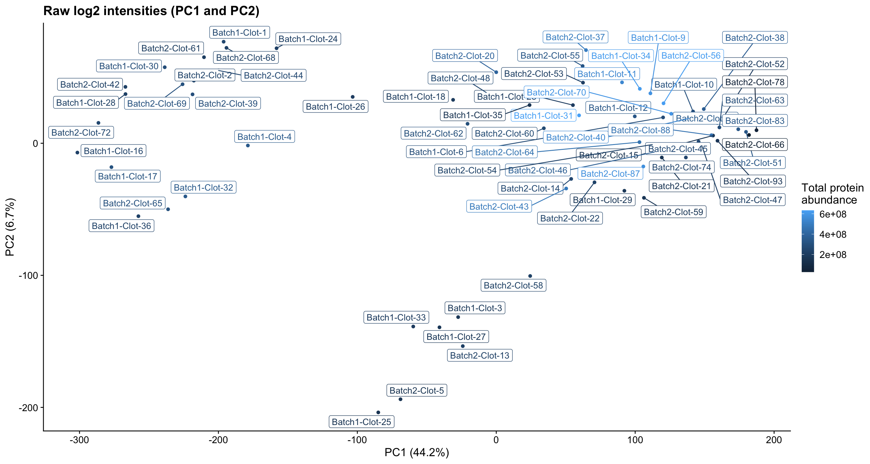
pc_analysis_raw$x %>%
  as.data.frame %>%
  rownames_to_column("sample") %>%
  dplyr::select(sample, PC1, PC3) %>%
  left_join(dge$samples %>% rownames_to_column("sample"), by = "sample") %>%
  ggplot(aes(x = PC1, y = PC3, colour = lib.size, label = sample)) +
  geom_point(show.legend = TRUE) +
  ggrepel::geom_label_repel(show.legend = FALSE) +
  ggtitle("Raw log2 intensities (PC1 and PC3)") +
  labs(x = "PC1 (44.2%)", y = "PC3 (5.7%)", colour = "Total protein\nabundance") +
  theme_cowplot()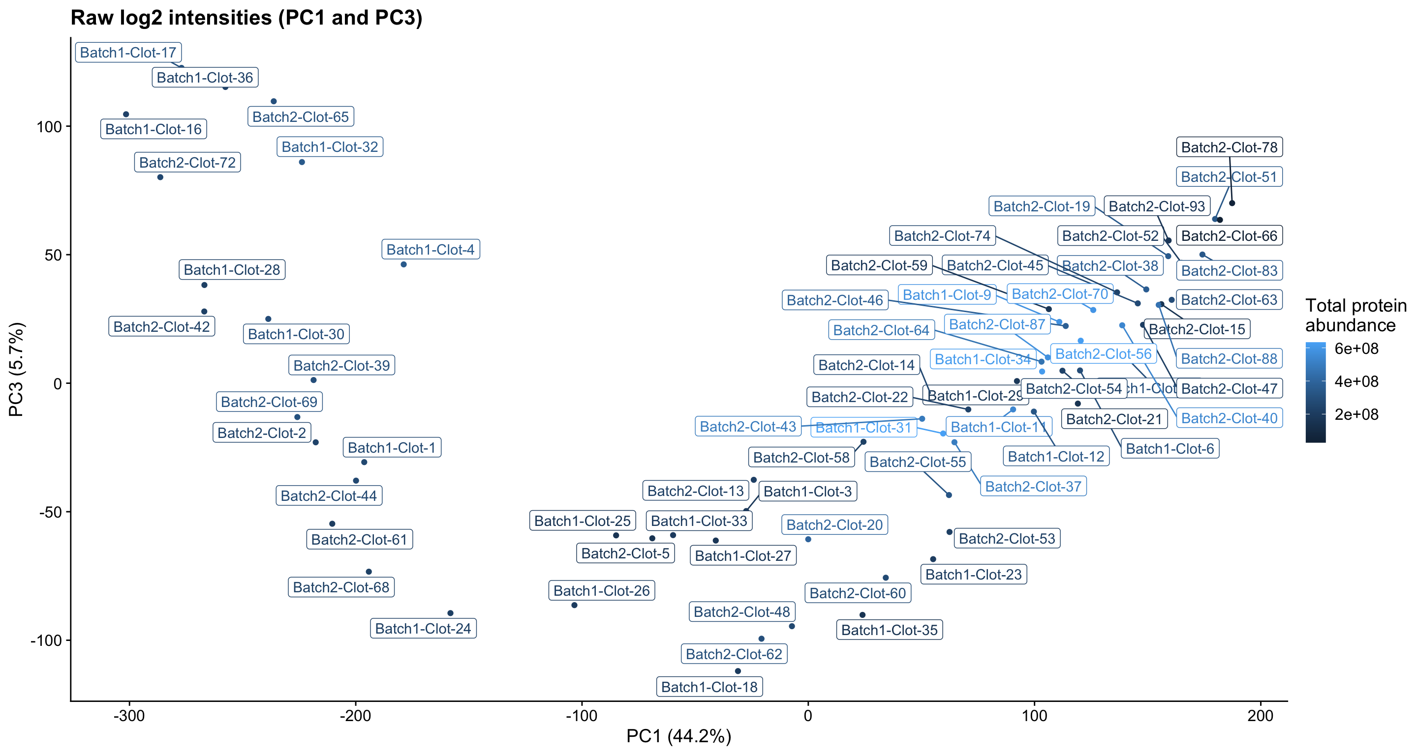
- After normalisation, most samples fall into one main cluster, with a few samples showing some extra variation. It is important to note that this variation is likely normal and not a cause of concern - especially as PC1 contributes only ~12% to the variation in protein abundances in the data.
pc_analysis_norm$x %>%
  as.data.frame %>%
  rownames_to_column("sample") %>%
  dplyr::select(sample, PC1, PC2) %>%
  left_join(dge$samples %>% rownames_to_column("sample"), by = "sample") %>%
  ggplot(aes(x = PC1, y = PC2, colour = lib.size, label = sample)) +
  geom_point(show.legend = FALSE) +
  ggrepel::geom_label_repel(show.legend = FALSE) +
  ggtitle("After Cyclic Loess Normalisation (PC1 and PC2)") +
  labs(x = "PC1 (12.2%)", y = "PC2 (9.3%)", colour = "Total protein\nabundance") +
  theme_cowplot()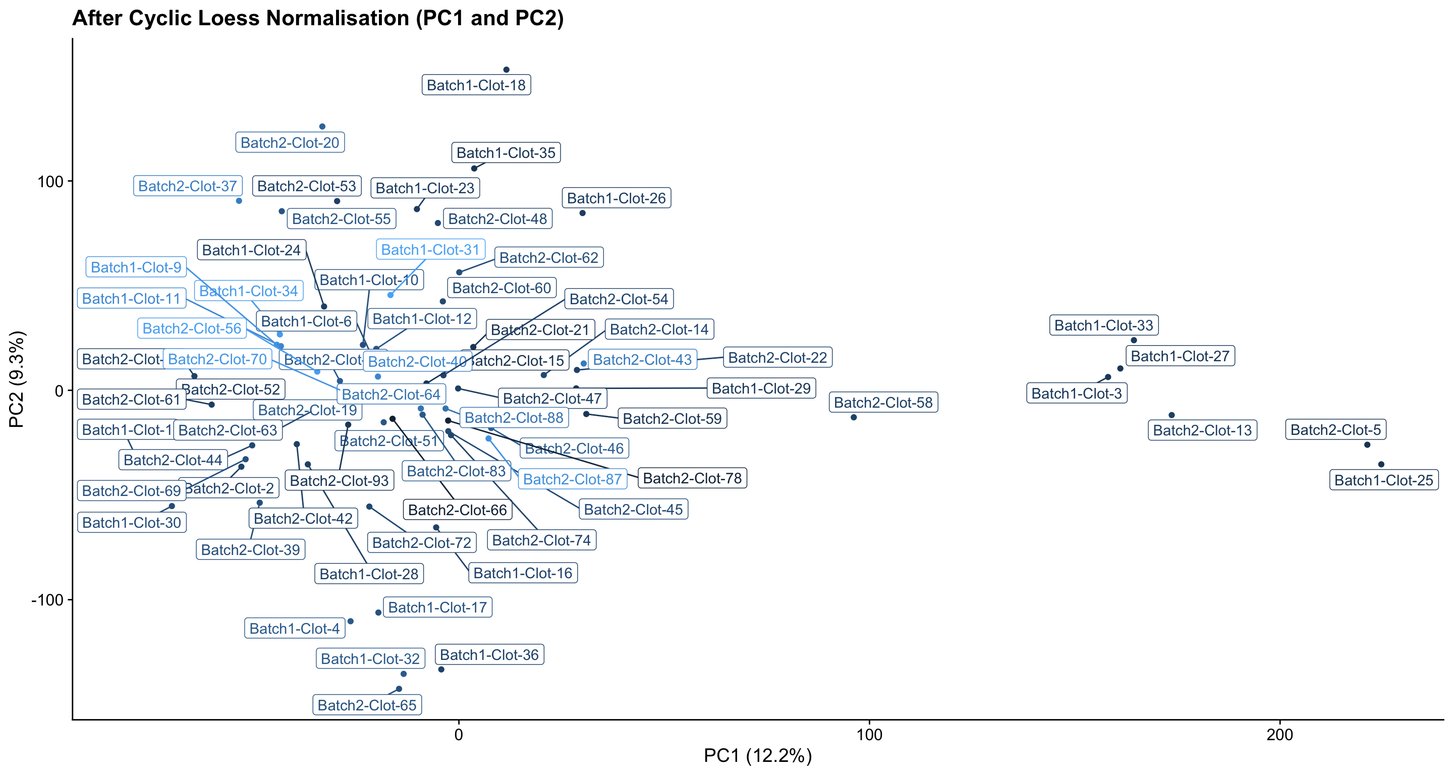
pc_analysis_norm$x %>%
  as.data.frame %>%
  rownames_to_column("sample") %>%
  dplyr::select(sample, PC1, PC3) %>%
  left_join(dge$samples %>% rownames_to_column("sample"), by = "sample") %>%
  ggplot(aes(x = PC1, y = PC3, colour = lib.size, label = sample)) +
  geom_point(show.legend = FALSE) +
  ggrepel::geom_label_repel(show.legend = FALSE) +
  ggtitle("After Cyclic Loess Normalisation (PC1 and PC3)") +
  labs(x = "PC1 (12.2%)", y = "PC3 (6.5%)", colour = "Total protein\nabundance") +
  theme_cowplot()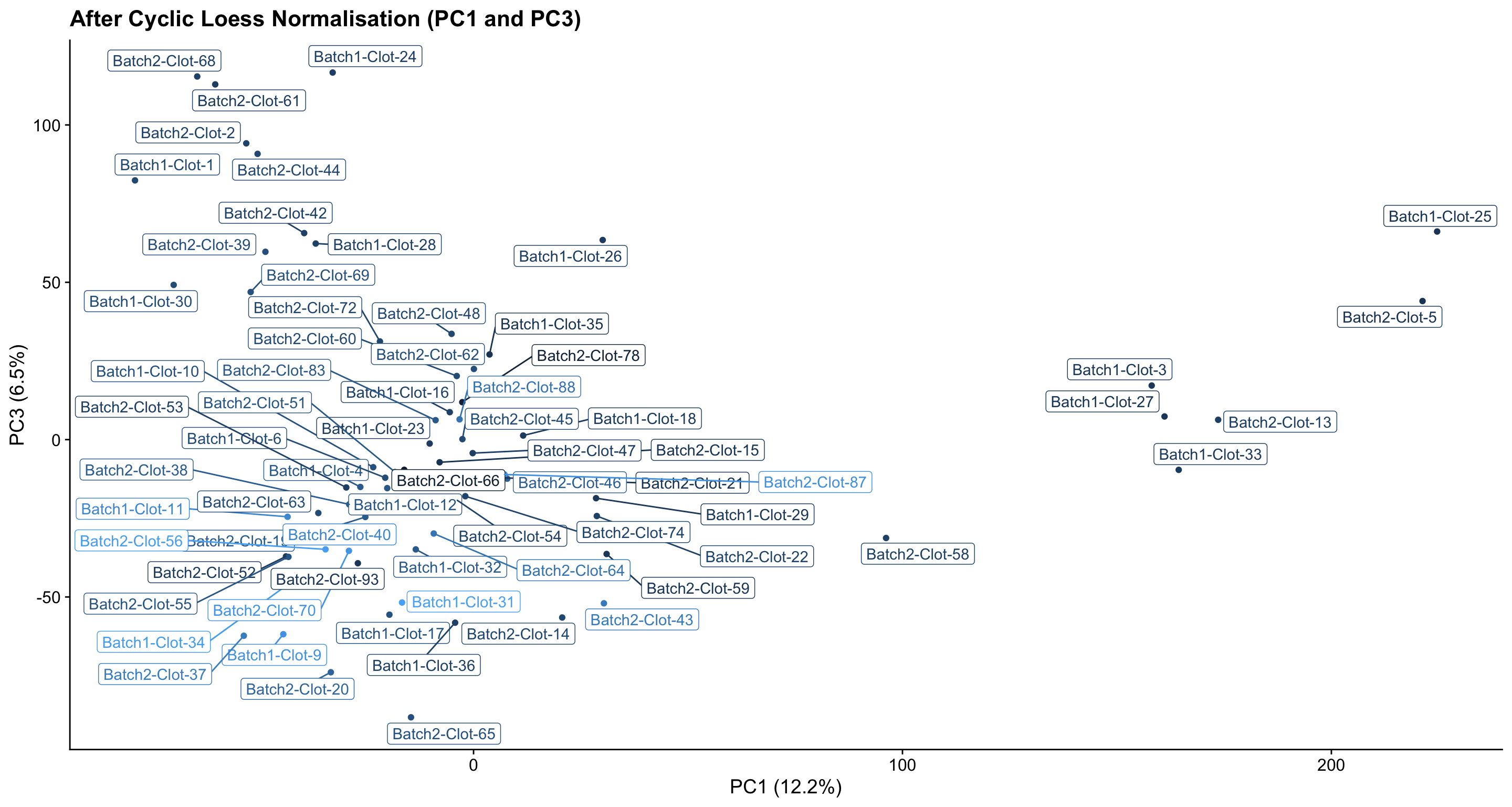
UMAP
PCA shows the global structure of the data well, but may not be the best at showing local structure. This may mean that subtle clustering in the data (eg differences between samples) may not stand out when PCA components are plotted. Here, I use a different dimension reduction technique UMAP which accounts for local structure. The idea behind UMAP is that it emphasises local structure at the cost of the distances between samples being representative of their overall similarity. (i.e. distances between samples are not directly proportional to how similar they are anymore).
Overall, the evidence suggests that distinct clusters in the data is unlikely based on the UMAP plot below (and PCAs above). Most samples appear to have fairly similar protein abundances, and there appears to be a normal amount of variation across the samples, with a few samples having more different protein abundances compared to the main group of samples.
umap_norm <- dge$norm %>% t %>% umap
umap_norm$layout %>%
  as.data.frame %>%
  rownames_to_column("sample") %>%
  dplyr::select(sample, V1, V2) %>%
  left_join(dge$samples %>% rownames_to_column("sample"), by = "sample") %>%
  #left_join(test ,by = "sample") %>%
  ggplot(aes(x = V1, y = V2, colour = lib.size, label = sample)) +
  geom_point(show.legend = FALSE) +
  ggrepel::geom_label_repel(show.legend = FALSE) +
  ggtitle("UMAP") +
  labs(x = "UMAP1", y = "UMAP2") +
  theme_cowplot()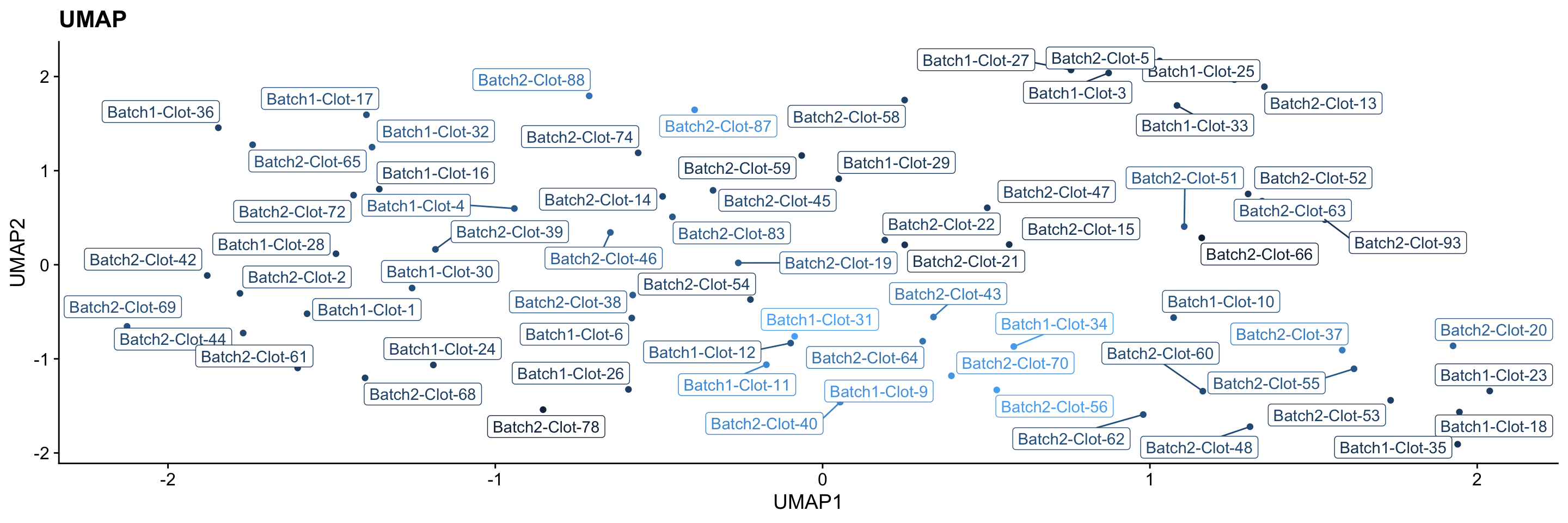
Contributors to variation in protein abundances (correlation between sample metadata variables)
Given that there is a decent amount variation in the samples even after normalisation, we may be interested in exploring the metadata which contributes to this variation. We can use a correlation plot as below to visualise the extent to which different sample metadata variables contribute to the first 5 PCs.
The Spearman correlations which are significant at the p-value < 0.1 level are shown below (the ones which are not significant are crossed out). Here we use Spearman correlation rather than Pearson as some of the variables are categorical (i.e. either 0 or 1) and not continuous.
The colour scale represents Spearman correlation (r^2) values.
importantFeatures <- dge$samples %>%
  rownames_to_column("sample") %>%
  #left_join(km_clusters, by = "sample") %>%
  dplyr::select_("sample",
                 "lib.size",
                "Age",
                "Sex",
                "Mechanism_Code",
                "Athero",
                "Smoking",
                "HTN",
                "AF",
                "Hyperlipidaemia",
                "Diabetes",
                "Prev_dx_of_stroke",
                "Prev_dx_of_TIA",
                "CHF",
                "IHD",
                "Aspirin",
                "Clopidogrel",
                "Dipyridamole",
                "Warfarin",
                "Other_antithrombotic",
                "Statin",
                "Suspended_Anticoagulant",
                "B_BG",
                "HbA1c_mmolL",
                "Cholesterol_1224hr",
                "Red_Cell_Count",
                "White_Cell_Count",
                "Platelet_Count",
                "Neutrophil_Count",
                "Thrombolysis",
                "Total_Passes",
                "Reocclusion"
                ) %>%
  dplyr::mutate(Sex = case_when(Sex == "F" ~ 0,
                                Sex == "M" ~ 1)) %>%
  dplyr::mutate(Sex = as.numeric(Sex)) %>%
  dplyr::rename(Total_Protein_Abundance = lib.size) %>%
  column_to_rownames("sample") %>%
    select_if(~ !any(is.na(.))) %>%
  dplyr::select(-Dipyridamole, -Warfarin)
Warning: `select_()` was deprecated in dplyr 0.7.0.
Please use `select()` instead.col3 <- colorRampPalette(c("red", "white", "SeaGreen"))
correlationDf <- importantFeatures %>%
rownames_to_column("sample") %>%
left_join(pc_analysis_norm$x %>%
as.data.frame %>%
rownames_to_column("sample") %>%
dplyr::select(sample, PC1, PC2, PC3, PC4, PC5)) %>%
column_to_rownames("sample") Joining, by = "sample"correlationDf <- sapply(correlationDf,as.numeric)
res1 <- corrplot::cor.mtest(correlationDf, conf.level = .95)
correlationDf %>%
cor(method = "spearman") %>%
corrplot::corrplot(
hclust.method = "average",
tl.col = "black",
tl.cex = 0.6,
#method = "number",
addgrid.col = "#eeeeee",
cl.ratio = .2,
cl.align = "l",
col = col3(20),
type = "upper",
p.mat = res1$p, sig.level = 0.1
)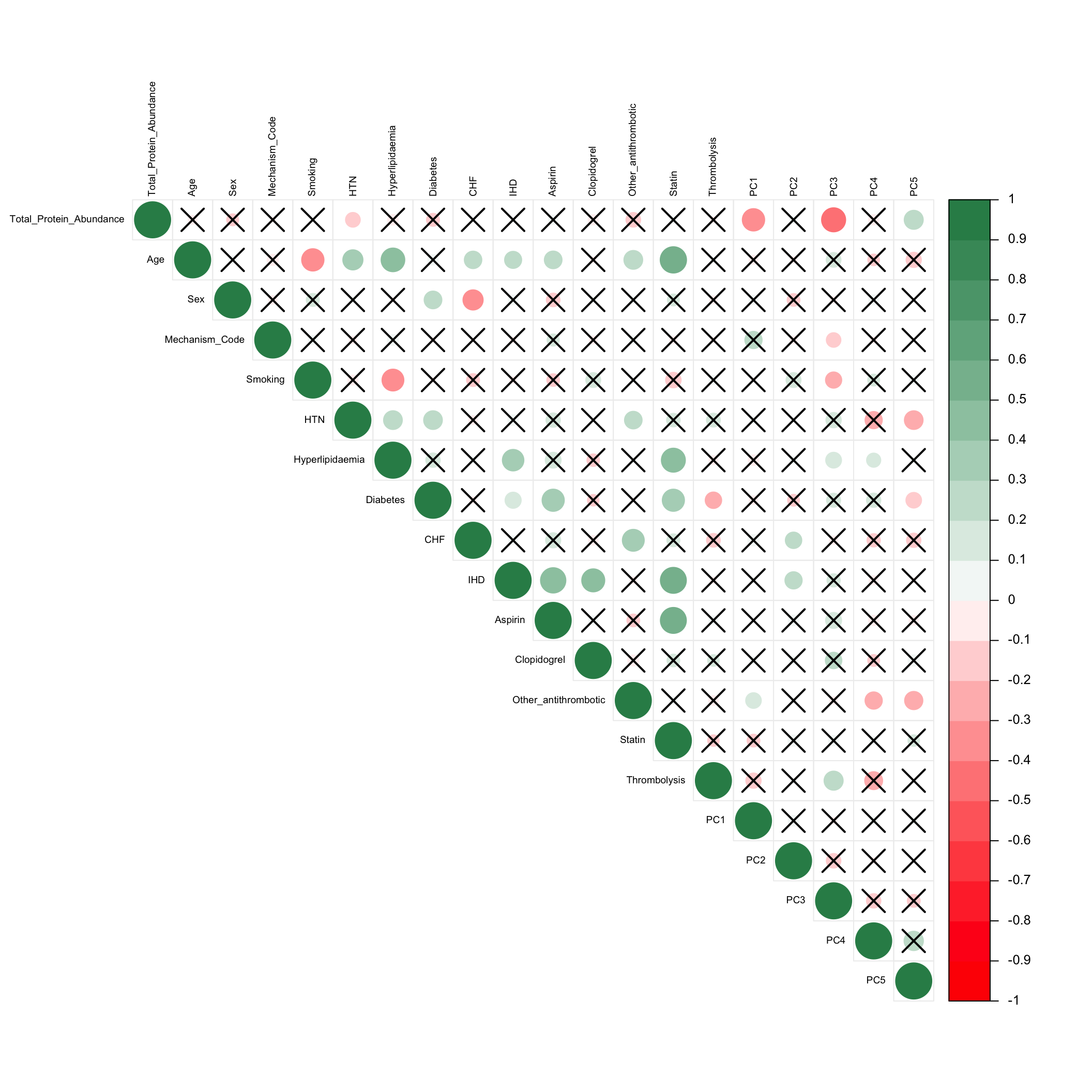
Overall, the variables are for the most part, not that correlated to each other. Correlation mainly ranges from -0.5 to 0.5.
The total protein abundance is the major source of variation in the data, showing significant correlation to both PC1 and PC3.
Many of the other metadata variables are correlated to Age (e.g. Smoking has negative correlation, HTN and Hyperlipidaemia are positively correlated)
Statin is also positively correlated to various other variables including Age, Hyperlipidaemia, Diabetes, IHD and Aspirin. However, all of these are either 0.5 or below, indicating the correlation is not extremely strong.
Not many of the biologically interesting variables are clearly correlated to any of the top 5 sources of variation in the data. This is concerning as it means that the biological effect on the protein abundances may be quite subtle, and difficult to detect/analyse.
Feature Importance
Another alternative to doing correlations between all metadata variables is to rank the variables by their feature importance. To do this, we build a model (here in the
caretpackage, the default is Random Forest (rf)), and then see which of the features are most informative for predicting a particular response variable.Below, I have set the response variable as
Mechanism_Codewhich corresponds to the mechanism (subtype) for the blood clot (a clinical diagnosis that we would expect to have quite a large effect in the data), and the features as the other variables in the correlation matrix above.We can see in the Feature Importance plot below that Age and Total_Protein_Abundance for each sample are the most important features, although Sex, Aspirin, Smoking, Statin, Diabetes etc also contribute a smaller amount of importance.
featuresToTest <- correlationDf %>%
  as.data.frame %>%
  dplyr::select(-starts_with("PC")) %>%
  as.matrix

control <- trainControl(method="repeatedcv", number=10, repeats=3)
# train the model
model <- train(Mechanism_Code~., data=featuresToTest,  preProcess="scale", trControl=control)
Warning in randomForest.default(x, y, mtry = param$mtry, ...): The response has
five or fewer unique values. Are you sure you want to do regression?
Warning in randomForest.default(x, y, mtry = param$mtry, ...): The response has
five or fewer unique values. Are you sure you want to do regression?
Warning in randomForest.default(x, y, mtry = param$mtry, ...): The response has
five or fewer unique values. Are you sure you want to do regression?
Warning in randomForest.default(x, y, mtry = param$mtry, ...): The response has
five or fewer unique values. Are you sure you want to do regression?
Warning in randomForest.default(x, y, mtry = param$mtry, ...): The response has
five or fewer unique values. Are you sure you want to do regression?
Warning in randomForest.default(x, y, mtry = param$mtry, ...): The response has
five or fewer unique values. Are you sure you want to do regression?
Warning in randomForest.default(x, y, mtry = param$mtry, ...): The response has
five or fewer unique values. Are you sure you want to do regression?
Warning in randomForest.default(x, y, mtry = param$mtry, ...): The response has
five or fewer unique values. Are you sure you want to do regression?
Warning in randomForest.default(x, y, mtry = param$mtry, ...): The response has
five or fewer unique values. Are you sure you want to do regression?
Warning in randomForest.default(x, y, mtry = param$mtry, ...): The response has
five or fewer unique values. Are you sure you want to do regression?
Warning in randomForest.default(x, y, mtry = param$mtry, ...): The response has
five or fewer unique values. Are you sure you want to do regression?
Warning in randomForest.default(x, y, mtry = param$mtry, ...): The response has
five or fewer unique values. Are you sure you want to do regression?
Warning in randomForest.default(x, y, mtry = param$mtry, ...): The response has
five or fewer unique values. Are you sure you want to do regression?
Warning in randomForest.default(x, y, mtry = param$mtry, ...): The response has
five or fewer unique values. Are you sure you want to do regression?
Warning in randomForest.default(x, y, mtry = param$mtry, ...): The response has
five or fewer unique values. Are you sure you want to do regression?
Warning in randomForest.default(x, y, mtry = param$mtry, ...): The response has
five or fewer unique values. Are you sure you want to do regression?
Warning in randomForest.default(x, y, mtry = param$mtry, ...): The response has
five or fewer unique values. Are you sure you want to do regression?
Warning in randomForest.default(x, y, mtry = param$mtry, ...): The response has
five or fewer unique values. Are you sure you want to do regression?# estimate variable importance
importance <- varImp(model, scale=FALSE)
# summarize importance
print(importance)rf variable importance
Overall
Age 52.915
Total_Protein_Abundance 47.191
Sex 6.760
Hyperlipidaemia 5.499
Aspirin 4.701
Smoking 3.983
HTN 3.077
Thrombolysis 2.946
Diabetes 2.601
Other_antithrombotic 2.579
Statin 2.551
IHD 2.278
Clopidogrel 1.591
CHF 1.056# plot importance
plot(importance)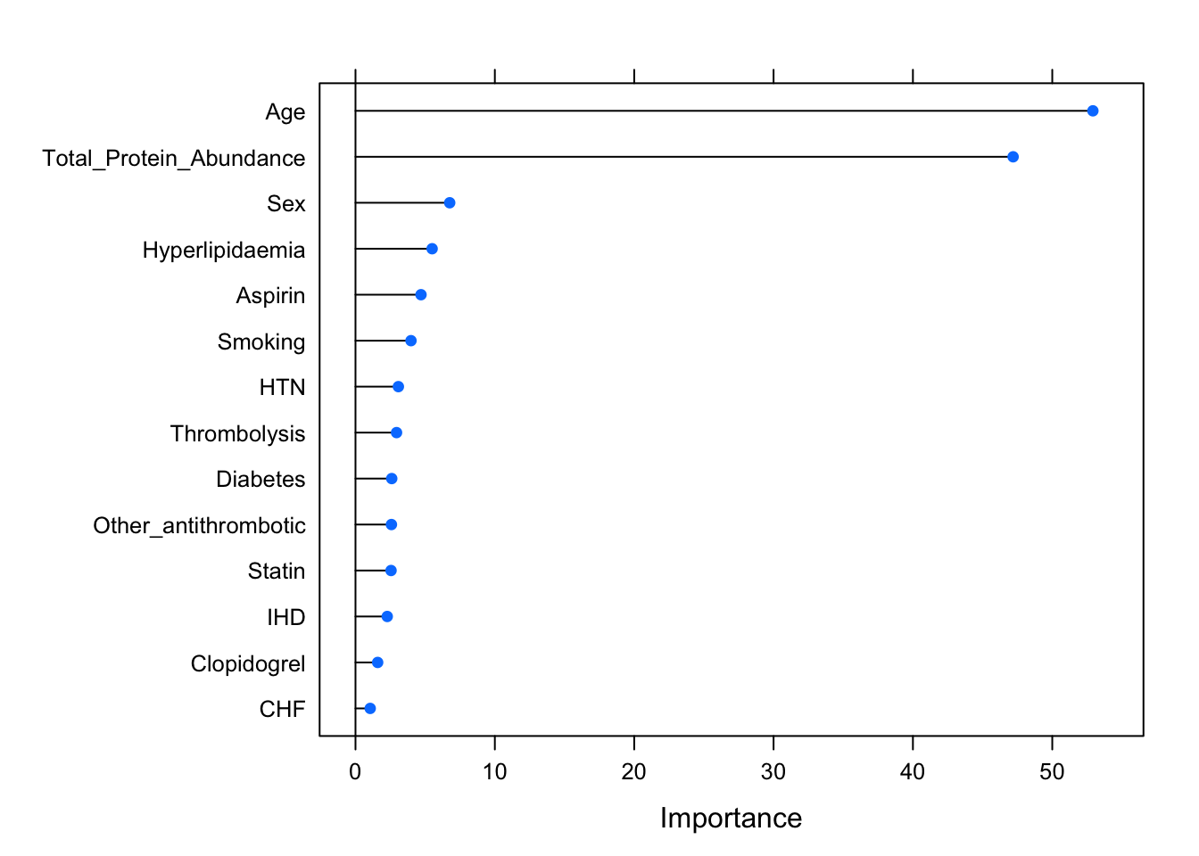
Proteins with High Expression
- I have gone through each sample and selected the top 10 most abundant proteins detected in each sample. A table is shown below, showing some of these proteins.
ncorresponds to how many samples have that protein as one of their top 10 most abundant proteins.
topExpressedProteins <- dge$norm %>%
  melt() %>%
  dplyr::group_by(Var2) %>%
  dplyr::arrange(desc(value), .by_group = TRUE) %>%
  dplyr::slice_max(order_by = value, n = 10) %>%
  inner_join(dge$genes, by = c("Var1"="UniProt_ID")) %>%
  dplyr::group_by(Var1) %>%
  dplyr::mutate(dupl = n() > 1)%>%
  dplyr::filter(dupl == TRUE) %>%
  dplyr::select(Var1, Var2, value, Protein_IDs, dupl)

topExpressedProteins2 <- topExpressedProteins %>%
  dplyr::summarise(n = n()) %>%
  dplyr::arrange(desc(n)) %>%
  dplyr::rename(UniProt_ID = Var1) %>%
  left_join(dge$genes[,c("UniProt_ID", "Gene")]) %>%
  dplyr::select(UniProt_ID, Gene, n)
Joining, by = "UniProt_ID"topExpressedProteins2# A tibble: 99 x 3
UniProt_ID Gene n
<chr> <chr> <int>
1 P69905 HBA 57
2 P68871 HBB 51
3 P60709 ACTB 41
4 P02671 FIBA 38
5 P02768 ALBU 35
6 P02675 FIBB 33
7 P02679 FIBG 33
8 P00915 CAH1 29
9 P21333 FLNA 26
10 P35579 MYH9 16
# … with 89 more rowsHeatmap visualisation
- A heatmap is used to visualise relative abundances of the most abundant proteins, along with relevant metadata variables.
# Create an annotation data.frame for the heatmap
# annot_cols <- dge$samples %>%
#   rownames_to_column("sample") %>%
#   dplyr::select(sample, Age, Sex, Mechanism_Code) %>%
#   column_to_rownames("sample")

annot_cols <- importantFeatures <- dge$samples %>%
  rownames_to_column("sample") %>%
  dplyr::select_("sample",
                 "lib.size",
                "Age",
                "Sex",
                "Mechanism_Code",
                "Athero",
                "Smoking",
                "HTN",
                "AF",
                "Hyperlipidaemia",
                "Diabetes",
                "Prev_dx_of_stroke",
                "Prev_dx_of_TIA",
                "CHF",
                "IHD",
                "Aspirin",
                "Clopidogrel",
                "Dipyridamole",
                "Warfarin",
                "Other_antithrombotic",
                "Statin",
                "Suspended_Anticoagulant",
                "B_BG",
                "HbA1c_mmolL",
                "Cholesterol_1224hr",
                "Red_Cell_Count",
                "White_Cell_Count",
                "Platelet_Count",
                "Neutrophil_Count",
                "Thrombolysis",
                "Total_Passes",
                "Reocclusion"
                ) %>%
  dplyr::rename(Total_Protein_Abundance = lib.size) %>%
  column_to_rownames("sample") %>%
    select_if(~ !any(is.na(.))) %>%
  dplyr::select(-Dipyridamole, -Warfarin)

annot_colours <- list(
  Smoking = c("0" = "#dddddd", "1" = "orange", "2" = "red"),
  Other_antithrombotic = c("0" = "#dddddd", "1" = "orange", "2" = "red"),
  Clopidogrel = c("0" = "#dddddd", "1" = "red"),
  Aspirin = c("0" = "#dddddd", "1" = "red"),
  IHD = c("0" = "#dddddd", "1" = "red"),
  CHF = c("0" = "#dddddd", "1" = "red"),
  Diabetes = c("0" = "#dddddd", "1" = "red"),
  HTN = c("0" = "#dddddd", "1" = "red"),
  Hyperlipidaemia = c("0" = "#dddddd", "1" = "red"),
  Thrombolysis = c("0" = "#dddddd", "1" = "red"),
  Statin = c("0" = "#dddddd", "1" = "red"),
  Mechanism_Code = c("0" = "Magenta",
                     "1" = "MediumPurple",
                     "2" = "turquoise",
                     "3" = "yellow",
                     "4" = "firebrick",
                     "5" = "YellowGreen"),
  Sex = c("M" = "royalblue", "F" = "salmon")
)


dataForHeatmap <- dge$norm %>%
  as.data.frame %>%
  rownames_to_column("UniProt_ID") %>%
  dplyr::filter(UniProt_ID %in% topExpressedProteins2$UniProt_ID) %>%
  left_join(topExpressedProteins2[, c("UniProt_ID", "Gene")]) %>%
  dplyr::mutate(Gene = paste0(Gene, " (", UniProt_ID, ")")) %>%
  dplyr::select(-UniProt_ID) %>%
  column_to_rownames("Gene")
Joining, by = "UniProt_ID"topAbundantProteinHeatmap <- dataForHeatmap %>%
pheatmap::pheatmap(scale="row", cellwidth = 10, cellheight=10,
color = colorRampPalette(c("#10c1e5",
"#82e0b4",
"#F9F9F9",
"#FBB829",
"#FF0066"))(100),
annotation_colors = annot_colours,
annotation_col = annot_cols,
border_color = "white",
treeheight_row = 0)
topAbundantProteinHeatmap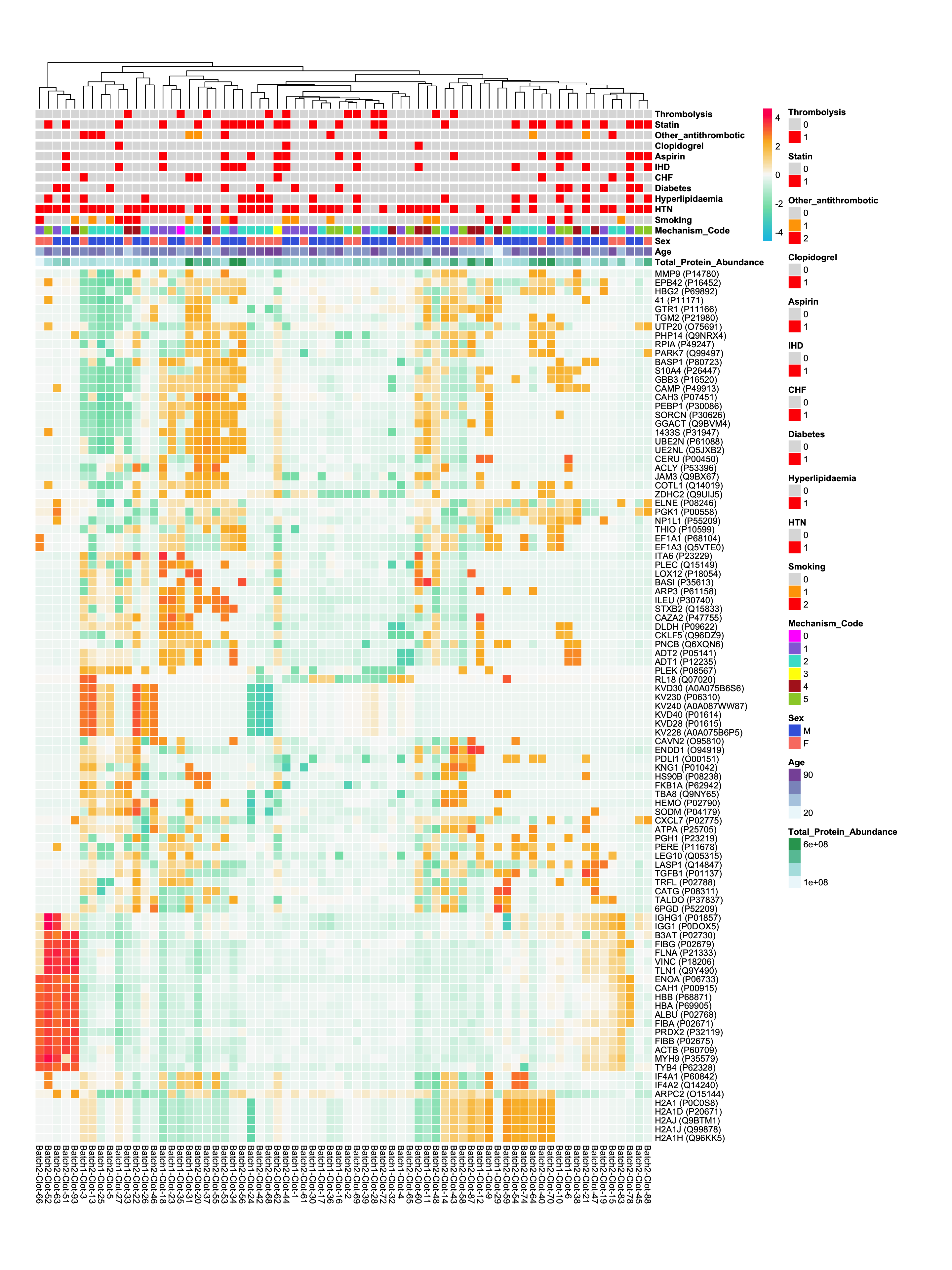
#save_pheatmap_pdf(topAbundantProteinHeatmap,
 #                 filename = here("output", "abundant_protein_heatmap.pdf"), width = 16, height = 20)
Highly Variable Proteins
- Here, I define Highly Variable proteins as those which are in the top 25% percentile of proteins showing the highest standard deviation across all samples and also are expressed at an abundance in the top 50% percentile of proteins.
variableProteins <- genefilter::rowSds(dge$norm) > quantile(genefilter::rowSds(dge$norm), 0.75)
table(variableProteins)
variableProteins
FALSE TRUE
1033 344 abundantProteins <- rowSums(dge$norm) > quantile(rowSums(dge$norm), 0.5)
table(abundantProteins)abundantProteins
FALSE TRUE
689 688 table(variableProteins & abundantProteins)
FALSE  TRUE
 1053   324
variableHeatmap <- dge$norm[(variableProteins & abundantProteins),] %>%
as.data.frame %>%
rownames_to_column("UniProt_ID") %>%
dplyr::left_join(dge$genes[, c("UniProt_ID", "Gene")]) %>%
dplyr::mutate(Gene = paste0(Gene, " (", UniProt_ID, ")")) %>%
dplyr::select(-UniProt_ID) %>%
column_to_rownames("Gene") %>%
pheatmap::pheatmap(scale="row",
cellwidth = 10, cellheight=10,
color = colorRampPalette(c("#10c1e5",
"#82e0b4",
"#F9F9F9",
"#FBB829",
"#FF0066"))(100),
annotation_colors = annot_colours,
annotation_col = annot_cols,
border_color = "white",
treeheight_row = 0)Joining, by = "UniProt_ID"variableHeatmap
#save_pheatmap_pdf(variableHeatmap,
#                  filename = here("output", "variable_protein_heatmap.pdf"), width = 16, height = 60)
topExpressedProteins <- dge$norm %>%
melt() %>%
dplyr::group_by(Var2) %>%
dplyr::arrange(desc(value), .by_group = TRUE) %>%
dplyr::slice_max(order_by = value, n = 10) %>%
inner_join(dge$genes, by = c("Var1"="UniProt_ID")) %>%
dplyr::group_by(Var1) %>%
dplyr::mutate(dupl = n() > 1)%>%
dplyr::filter(dupl == TRUE) %>%
dplyr::select(Var1, Var2, value, Protein_IDs, dupl)
topExpressedProteins2 <- topExpressedProteins %>%
dplyr::summarise(n = n()) %>%
dplyr::arrange(desc(n)) %>%
dplyr::rename(UniProt_ID = Var1) %>%
left_join(dge$genes[,c("UniProt_ID", "Gene")]) %>%
dplyr::select(UniProt_ID, Gene, n)Joining, by = "UniProt_ID"topExpressedProteins2# A tibble: 99 x 3
UniProt_ID Gene n
<chr> <chr> <int>
1 P69905 HBA 57
2 P68871 HBB 51
3 P60709 ACTB 41
4 P02671 FIBA 38
5 P02768 ALBU 35
6 P02675 FIBB 33
7 P02679 FIBG 33
8 P00915 CAH1 29
9 P21333 FLNA 26
10 P35579 MYH9 16
# … with 89 more rowsNext steps
- Unfortunately, the story that the data tells us is that the majority of variation seen in protein abundances between samples cannot be explained by the vast majority of the metadata variables that were measured for the samples. Possible reasons for this may include:
Technical artifacts or “batch effects” in samples: Blood clot samples were not all taken on the same day, and their protein abundances were measured on different days. This can cause a technical batch effect where differences in storage time / wet-lab differences etc could contribute to the majority of variation we are seeing. Because the date at which protein abundances and other metadata variables were measured is not available, we cannot try to correct for this batch effect statistically (e.g. through modelling it as a fixed effect in a linear model). For all future samples which are collected, it is important that we include the dates / batches of when they were processed / measured.
Possible insufficient sample size: There are 70 samples representing 5 different types of blood clots. Some of the types of blood clot do not have many samples and this may not be representative of the protein abundances. A greater sample size would likely be very helpful in seeing how strong the true biological effect is vs. technical artifacts.
Missing and incorrectly coded data in sample metadata: Some of the sample metadata is incomplete (missing values) or incorrectly/inconsistently coded.
sessionInfo()R version 4.0.3 (2020-10-10)
Platform: x86_64-apple-darwin17.0 (64-bit)
Running under: macOS Mojave 10.14.6
Matrix products: default
BLAS: /Library/Frameworks/R.framework/Versions/4.0/Resources/lib/libRblas.dylib
LAPACK: /Library/Frameworks/R.framework/Versions/4.0/Resources/lib/libRlapack.dylib
locale:
[1] en_AU.UTF-8/en_AU.UTF-8/en_AU.UTF-8/C/en_AU.UTF-8/en_AU.UTF-8
attached base packages:
[1] grid parallel stats4 stats graphics grDevices utils
[8] datasets methods base
other attached packages:
[1] umap_0.2.7.0 pheatmap_1.0.12 cowplot_1.1.0
[4] mlbench_2.1-3 caret_6.0-86 lattice_0.20-41
[7] org.Hs.eg.db_3.12.0 AnnotationDbi_1.52.0 IRanges_2.24.0
[10] S4Vectors_0.28.0 Biobase_2.50.0 BiocGenerics_0.36.0
[13] edgeR_3.32.0 limma_3.46.0 readr_1.4.0
[16] tidyr_1.1.3 tibble_3.1.1 reshape2_1.4.4
[19] ggplot2_3.3.3 dplyr_1.0.5 magrittr_2.0.1
[22] here_1.0.0 workflowr_1.6.2
loaded via a namespace (and not attached):
[1] nlme_3.1-149 fs_1.5.0 lubridate_1.7.10
[4] bit64_4.0.5 httr_1.4.2 RColorBrewer_1.1-2
[7] rprojroot_2.0.2 tools_4.0.3 bslib_0.2.4
[10] utf8_1.1.4 R6_2.5.0 rpart_4.1-15
[13] DBI_1.1.0 colorspace_2.0-0 nnet_7.3-14
[16] withr_2.3.0 tidyselect_1.1.0 bit_4.0.4
[19] compiler_4.0.3 git2r_0.27.1 cli_3.0.1
[22] labeling_0.4.2 sass_0.3.1 scales_1.1.1
[25] genefilter_1.72.1 randomForest_4.6-14 askpass_1.1
[28] stringr_1.4.0 digest_0.6.27 rmarkdown_2.8
[31] pkgconfig_2.0.3 htmltools_0.5.1.1 rlang_0.4.10
[34] rstudioapi_0.13 RSQLite_2.2.1 farver_2.0.3
[37] jquerylib_0.1.3 generics_0.1.0 jsonlite_1.7.2
[40] ModelMetrics_1.2.2.2 Matrix_1.2-18 Rcpp_1.0.5
[43] munsell_0.5.0 fansi_0.4.1 reticulate_1.18
[46] lifecycle_1.0.0 stringi_1.5.3 whisker_0.4
[49] pROC_1.16.2 yaml_2.2.1 MASS_7.3-53
[52] plyr_1.8.6 recipes_0.1.15 blob_1.2.1
[55] ggrepel_0.8.2 promises_1.1.1 crayon_1.4.1
[58] splines_4.0.3 annotate_1.68.0 hms_1.0.0
[61] locfit_1.5-9.4 knitr_1.30 pillar_1.6.0
[64] codetools_0.2-16 XML_3.99-0.5 glue_1.4.2
[67] evaluate_0.14 data.table_1.13.2 vctrs_0.3.7
[70] httpuv_1.5.4 foreach_1.5.1 openssl_1.4.3
[73] gtable_0.3.0 purrr_0.3.4 assertthat_0.2.1
[76] xfun_0.23 gower_0.2.2 prodlim_2019.11.13
[79] xtable_1.8-4 RSpectra_0.16-0 later_1.1.0.1
[82] class_7.3-17 survival_3.2-7 timeDate_3043.102
[85] iterators_1.0.13 memoise_1.1.0 corrplot_0.84
[88] lava_1.6.8.1 ellipsis_0.3.1 ipred_0.9-9